import pandas as pd
import numpy as np
import matplotlib.pyplot as plt
import seaborn as sns
from numpy.random import default_rng8 Intro to Models
In this lecture we will learn about modeling data for the first time. After this lesson, you should know what we generally mean by a “model”, what linear regression is and how to interpret the output. But first we need to introduce a new data type: categorical variables.
Online Resources:
Chapter 7.5 of our textbook introduces categorical variables.
import statsmodels.api as sm
import statsmodels.formula.api as smf
#!pip install gapminder
from gapminder import gapmindergapminder.head()| country | continent | year | lifeExp | pop | gdpPercap | |
|---|---|---|---|---|---|---|
| 0 | Afghanistan | Asia | 1952 | 28.801 | 8425333 | 779.445314 |
| 1 | Afghanistan | Asia | 1957 | 30.332 | 9240934 | 820.853030 |
| 2 | Afghanistan | Asia | 1962 | 31.997 | 10267083 | 853.100710 |
| 3 | Afghanistan | Asia | 1967 | 34.020 | 11537966 | 836.197138 |
| 4 | Afghanistan | Asia | 1972 | 36.088 | 13079460 | 739.981106 |
Categorical variables
As a motivation, take another look at the gapminder data which contains variables of a mixed type: numeric columns along with string type columns which contain repeated instances of a smaller set of distinct or discrete values which
- are not numeric (but could be represented as numbers)
- cannot really be ordered
- typically take on a finite set of values, or categories.
We refer to these data types as categorical.
We have already seen functions like unique and value_counts, which enable us to extract the distinct values from an array and compute their frequencies.
Boxplots and grouping operations typically use a categorical variable to compute summaries of a numerical variables for each category separately, e.g.
gapminder.boxplot(column = "lifeExp", by="continent",figsize=(5, 2));
plt.title('Life expectancy by continent')
# Remove the default suptitle
plt.suptitle("");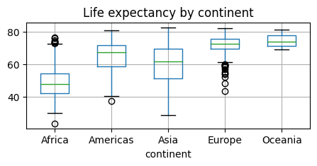
pandas has a special Categorical extension type for holding data that uses the integer-based categorical representation or encoding. This is a popular data compression technique for data with many occurrences of similar values and can provide significantly faster performance with lower memory use, especially for string data.
gapminder.info()<class 'pandas.core.frame.DataFrame'>
RangeIndex: 1704 entries, 0 to 1703
Data columns (total 6 columns):
# Column Non-Null Count Dtype
--- ------ -------------- -----
0 country 1704 non-null object
1 continent 1704 non-null object
2 year 1704 non-null int64
3 lifeExp 1704 non-null float64
4 pop 1704 non-null int64
5 gdpPercap 1704 non-null float64
dtypes: float64(2), int64(2), object(2)
memory usage: 80.0+ KBgapminder['country'] = gapminder['country'].astype('category')
gapminder.info()<class 'pandas.core.frame.DataFrame'>
RangeIndex: 1704 entries, 0 to 1703
Data columns (total 6 columns):
# Column Non-Null Count Dtype
--- ------ -------------- -----
0 country 1704 non-null category
1 continent 1704 non-null object
2 year 1704 non-null int64
3 lifeExp 1704 non-null float64
4 pop 1704 non-null int64
5 gdpPercap 1704 non-null float64
dtypes: category(1), float64(2), int64(2), object(1)
memory usage: 75.2+ KBWe will come back to the usefulness of this later.
Tables as models
For now let us look at our first “model”:
titanic = sns.load_dataset('titanic')
titanic["class3"] = (titanic["pclass"]==3)
titanic["male"] = (titanic["sex"]=="male")
titanic.head()| survived | pclass | sex | age | sibsp | parch | fare | embarked | class | who | adult_male | deck | embark_town | alive | alone | class3 | male | |
|---|---|---|---|---|---|---|---|---|---|---|---|---|---|---|---|---|---|
| 0 | 0 | 3 | male | 22.0 | 1 | 0 | 7.2500 | S | Third | man | True | NaN | Southampton | no | False | True | True |
| 1 | 1 | 1 | female | 38.0 | 1 | 0 | 71.2833 | C | First | woman | False | C | Cherbourg | yes | False | False | False |
| 2 | 1 | 3 | female | 26.0 | 0 | 0 | 7.9250 | S | Third | woman | False | NaN | Southampton | yes | True | True | False |
| 3 | 1 | 1 | female | 35.0 | 1 | 0 | 53.1000 | S | First | woman | False | C | Southampton | yes | False | False | False |
| 4 | 0 | 3 | male | 35.0 | 0 | 0 | 8.0500 | S | Third | man | True | NaN | Southampton | no | True | True | True |
vals1, cts1 = np.unique(titanic["class3"], return_counts=True)
print(cts1)
print(vals1)
[400 491]
[False True]print("The mean survival on the Titanic was", np.mean(titanic.survived))The mean survival on the Titanic was 0.3838383838383838ConTbl = pd.crosstab(titanic["sex"], titanic["survived"])
ConTbl| survived | 0 | 1 |
|---|---|---|
| sex | ||
| female | 81 | 233 |
| male | 468 | 109 |
What are the estimated survival probabilities?
#the good old groupby way:
bySex = titanic.groupby("sex").survived
bySex.mean()
sex
female 0.742038
male 0.188908
Name: survived, dtype: float64p3D = pd.crosstab([titanic["sex"], titanic["class3"]], titanic["survived"])
p3D| survived | 0 | 1 | |
|---|---|---|---|
| sex | class3 | ||
| female | False | 9 | 161 |
| True | 72 | 72 | |
| male | False | 168 | 62 |
| True | 300 | 47 |
What are the estimated survival probabilities?
#the good old groupby way:
bySex = titanic.groupby(["sex", "class3"]).survived
bySex.mean()
sex class3
female False 0.947059
True 0.500000
male False 0.269565
True 0.135447
Name: survived, dtype: float64The above table can be looked at as a model, which is defined as a function which takes inputs x and “spits out” a prediction:
\(y = f(\mathbf{x})\)
In our case, the inputs are \(x_1=\text{sex}\), \(x_2=\text{class3}\), and the output is the estimated survival probability!
It is evident that we could keep adding more input variables and make finer and finer grained predictions.
Linear Models
lsFit = smf.ols('survived ~ sex:class3-1', titanic).fit()
lsFit.summary().tables[1]| coef | std err | t | P>|t| | [0.025 | 0.975] | |
|---|---|---|---|---|---|---|
| sex[female]:class3[False] | 0.9471 | 0.029 | 32.200 | 0.000 | 0.889 | 1.005 |
| sex[male]:class3[False] | 0.2696 | 0.025 | 10.660 | 0.000 | 0.220 | 0.319 |
| sex[female]:class3[True] | 0.5000 | 0.032 | 15.646 | 0.000 | 0.437 | 0.563 |
| sex[male]:class3[True] | 0.1354 | 0.021 | 6.579 | 0.000 | 0.095 | 0.176 |
Modeling Missing Values
We have already seen how to detect and how to replace missing values. But the latter -until now- was rather crude: we often replaced all values with a “global” average.
Clearly, we can do better than replacing all missing entries in the survived column with the average \(0.38\).
rng = default_rng()

missingRows = rng.integers(0,890,20)
print(missingRows)
#introduce missing values
titanic.iloc[missingRows,0] = np.nan
np.sum(titanic.survived.isna())
[864 299 857 182 808 817 802 295 255 644 1 685 452 463 303 551 517 502
495 412]20predSurv = lsFit.predict()
print( len(predSurv))
predSurv[titanic.survived.isna()]891array([0.94705882, 0.13544669, 0.5 , 0.26956522, 0.94705882,
0.94705882, 0.94705882, 0.26956522, 0.26956522, 0.13544669,
0.5 , 0.13544669, 0.26956522, 0.5 , 0.26956522,
0.26956522, 0.26956522, 0.26956522, 0.26956522, 0.26956522])From categorical to numerical relations
url = "https://drive.google.com/file/d/1UbZy5Ecknpl1GXZBkbhJ_K6GJcIA2Plq/view?usp=share_link"
url='https://drive.google.com/uc?id=' + url.split('/')[-2]
auto = pd.read_csv(url)
auto.head()| mpg | cylinders | displacement | horsepower | weight | acceleration | year | origin | name | Manufacturer | |
|---|---|---|---|---|---|---|---|---|---|---|
| 0 | 18.0 | 8 | 307.0 | 130 | 3504 | 12.0 | 70 | 1 | chevrolet chevelle malibu | chevrolet |
| 1 | 15.0 | 8 | 350.0 | 165 | 3693 | 11.5 | 70 | 1 | buick skylark 320 | buick |
| 2 | 18.0 | 8 | 318.0 | 150 | 3436 | 11.0 | 70 | 1 | plymouth satellite | plymouth |
| 3 | 16.0 | 8 | 304.0 | 150 | 3433 | 12.0 | 70 | 1 | amc rebel sst | amc |
| 4 | 17.0 | 8 | 302.0 | 140 | 3449 | 10.5 | 70 | 1 | ford torino | ford |
plt.figure(figsize=(5,3))
plt.scatter(x=auto["weight"], y=auto["mpg"]);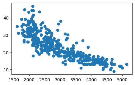
Linear Regression
We can roughly estimate, i.e. “model” this relationship with a straight line:
\[ y = \beta_0 + \beta_1 x \]
plt.figure(figsize=(5,3))
tmp=sns.regplot(x=auto["weight"], y=auto["mpg"], order=1, ci=95,
                scatter_kws={'color':'b', 's':9}, line_kws={'color':'r'})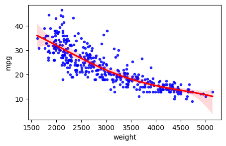
Remind yourself of the definition of the slope of a straight line
\[ \beta_1 = \frac{\Delta y}{\Delta x} = \frac{y_2-y_1}{x_2-x_1} \]
est = smf.ols('mpg ~ weight', auto).fit()
est.summary().tables[1]| coef | std err | t | P>|t| | [0.025 | 0.975] | |
|---|---|---|---|---|---|---|
| Intercept | 46.2165 | 0.799 | 57.867 | 0.000 | 44.646 | 47.787 |
| weight | -0.0076 | 0.000 | -29.645 | 0.000 | -0.008 | -0.007 |
np.corrcoef(auto["weight"], auto["mpg"])array([[ 1. , -0.83224421],
[-0.83224421, 1. ]])Further Reading: